R AND R-TAXBEN

Introduction
This slideshow is about a preliminary translation
of a simulation of the UK economy from Python into R. The simulation
is a “microeconomic” model, meaning that it simulates at the level
of individual people. In contrast, a “macroeconomic” model (which this
is not), would simulate bulk economic variables such as inflation and
unemployment.
The model reads surveys of households,
with their expenditure and income. To these, it applies rules
describing
the UK tax and benefits system. Users can change
these via a front-end: for example, increase VAT
on alcohol or decrease child benefit.
Using the rules,
it calculates how the changes would affect each household’s
net expenditure and income.
Introduction II
The model can use various different data sets.
For our initial translation, we’re concentrating
on the Government’s
Family
Resources Survey, which surveys
20,000 households each year. See
“Introduction
to the Family Resources Survey”
for an overview of the 2013-2014 survey. This
and other documentation, including details of the columns
in the data tables, are available
at the “Family
Resources Survey, 2013-2014”
data catalogue page.
Introduction III
Models like this can be used in various ways. One is evaluation of
Government economic policy. If the Government increases income tax,
how will this affect net incomes? Will it
push a lot of low-income people into poverty? Or will
it extract income mainly from the better off? To answer such questions,
we need to summarise how change affects the population
as a whole, via tools such as graphs of
income distribution.
Another use is education: about economics, about policy, and
about statistics and data analysis. I’ll say more about this
later. We believe it’s an important application, where
R will be very helpful.
Introduction IV: Credits
The work reported here was done in
R version
3.4.2, mainly
for
Windows. I used various packages, not
least
Hadley Wickham’s
Tidyverse.
Of which, I’ll have a lot more to say.
The microsimulation
model being translated was written
by
Landman
Economics. Funding for this proof-of-concept
was provided by Landman.
The R-Taxben
logo was derived from the
R logo, which is
available under the Creative
Commons Attribution-ShareAlike 4.0 International license (CC-BY-SA
4.0). It contains extra graphics surrounding the R logo, which
has not itself been changed.
About This Presentation
I’ve designed this slideshow to be the
closest thing I could make to a video
or to one side of a conversation. So
I’ve structured it as “fragments”, each being like a sentence
where I’m showing something new
or amplifying something already shown.
To progress through the fragments, press the right-arrow
control or right-arrow on the keyboard. Left-arrow will go
backwards, unshowing fragments one by one. Clicking the browser
background and typing O will toggle between the current slide
and a strip view of all the slides. Clicking on the
“contents” icon at top left will go to the contents page, slide 9.
Many slides contain screenshots. So that the text in
them is legible, use the biggest screen you can find.
I wrote this on a 23″ 1920×1080 pixel
screen, with the browser window roughly 1270 pixels by
850 pixels.
About This Presentation II
There are two versions of this presentation. One, which
I wrote for colleagues who don’t know R, is the
“fragments” one mentioned in the
previous slide.
The other is a
“non-fragments”
one which allows quicker reading. It makes each slide
come into view in one go. Its screenshots
come into view with the rest of their slide, and
are animated to cater for the fact that many of them scroll the
R window, and hence can’t be fitted into one
image.
To change views, use the links here, or those under the
contents icon.
Before reading the slideshow, you may like to
try my blog post
at “R-Taxben:
a Microsimulation Economic Model in R”.
About This Presentation III: Credits
This presentation was written in Hakim
El Hattab et. al.’s
reveal.js.
This is a JavaScript system for building
web-based slideshows. A demonstration
can be seen at
revealjs.com .
The contents page was implemented
with Frederick Feibel’s
Presentable
plugin.
Contents
What Is R?
R is a programming language for statistics, with
enough features to be useful for general-purpose
progranmming as well.
R programs can be run from the command-line, from
web servers, and from operating-system scripts. However,
R can also be run interactively.
R makes it easy to examine data and track down
errors and anomalies. Tools include
histograms, functions for counting and categorising,
and queries for sorting and filtering.
Why Use R?
R will (I hope) be able to program
everything we need.
… including all the stats and
graphics we could ever desire …
… and the tools for tracking down errors and
anomalies in data and results.
R will also (I hope) be fast enough.
R can be run from the web.
R has excellent packages for testing code.
R has an active user community, knowledgeable and
approachable developers, and a lot of high-quality
libraries.
Interactiveness will help users get
a feel for R-Taxben and its data.
A Glimpse of R: Interaction

A Glimpse of R: Variables

A Glimpse of R: Interaction II
In the screenshots, my input is in red.
The R prompt, >, is also in red,
but I never type that: R does.
R’s other output is in blue.

Sometimes, there is no output, such as after an assignment.
But usually, R displays a result. This is preceded by
a number in square brackets saying how many elements the result
contains. That’s because R treats even single numbers as vectors
and so feels compelled to tell you how long these are.
A Glimpse of R: Interaction III
In these slides, when you click right arrow or press the
right-arrow key, it displays a later version of the
screenshot. Generally, this shows one more piece of
input to R, and its result. So one more piece of
red and one more piece of blue. Occasionally, it shows
two pieces of input and the results.
In later screenshots, I may pause right after each
input, so that you get the effect of typing a command
and then seeing its result. That’s useful when
I’m demonstrating things like graphics where R pops up
new windows. But I thought doing that everywhere would
be annoying, because it needs you to click or press
more often.
A Glimpse of R: Functions

A Glimpse of R: Functions in Source Code
# Converts the year and month to a string
# of the form "2014-15" denoting the tax
# year starting in 'month' of 'year'.
# This function is vectorised.
#
year_and_month_to_tax_year <- function( year, month )
{
  firstyear <-
    ifelse( month <= 3, year-1, year )

  tax_year <-
    sprintf( '%04d-%02d', firstyear, ( firstyear + 1 ) %% 100 )

  tax_year
}
A Glimpse of R: Datatypes

R: The Same but Different
So R has things that you’d find in other
languages, including variables, functions,
conditionals, Booleans and strings. But it also
does some things slightly differently, and other
things very differently.
Example of a slight difference: paste (previous slide)
for joining strings.
Example of a big difference: vectors (also previous slide).
These differences mean translating code
literally from another language may not work, or work well.
And we must beware of faux amis.
The R Inferno
Some differences between R and other
languages are so big that there is an entire book warning
programmers about them. The R
Inferno by Patrick Burns.

The R Inferno II

(The Dante’s Inferno ride entrance in Panama City, Florida: by
“Marktippin”.)
So Again, Why Use R?
So if R is so weird, why use it?
I’ve mentioned its excellent stats and graphics, its
data-analysis tools, its interactivity, its tools for testing
code, its libraries and user community. But it also has a datatype which
matches the
structure of our data. I claim that, together with interactivity,
this will make the “things” that R-Taxben operates on seem
more real to its users.
Reification
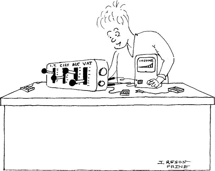
Programmers live their working lives surrounded by data structures and
subroutines, entities that grow to become as concrete
— as “thing-like”, as
“manipulable” — as teacups
and bricks.
The
feeling of thing-ness is strengthened, I believe, by interactive shells
such
as R’s which enable one to call functions and inspect their results, and
to store these in variables and pass them around. For R-Taxben, those
results are either chunks of economic data such as our tables of
households, or income-distribution graphs and other summaries. I hope
that being able to touch, probe, and pick up these things with R will make
them seem more real.
Reification II
Educational Microworlds
Educational microworlds, non-threatening
playgrounds where students learn by
experiment,
were popularised by
Seymour
Papert. He co-designed Logo, with which children
learned mathematics by programming “turtles” to
draw squares and other figures.
For an introduction, see
Education Week‘s
“Seymour
Papert’s ‘Microworld’: An Educational Utopia”.
There’s a survey of Logo and other microworlds in
Lloyd P. Rieber’s “Microworlds”. To
quote: “However, another, much smaller
collection of software, known as
microworlds,
is based on very different principles, those of invention,
play, and discovery. Instead of seeking to give students
knowledge passed down from one generation to the next as
efficiently as possible, the aim is to give students the resources to
build and refine their own knowledge in personal and meaningful ways.”
Educational Microworlds II
“Logo is the name for a philosophy of education and for a continually
evolving family of computer languages that aid its realization.
Its learning environments articulate the principle that giving people personal
control over powerful computational resources can enable them to
establish intimate contact with profound ideas from science,
from mathematics, and from the art of intellectual model building. Its computer
languages are designed to transform computers into
flexible tools to aid
in learning, in playing, and in exploring.”
From Logo for the Apple II by H. Abelson, quoted in Rieber.
Educational Microworlds III: Can We Build an EconomicsLand?
“Similar to the idea that the best way to learn Spanish is
to go and live in Spain, Papert conjectured that learning
mathematics via Logo was similar to having students visit a comput-
erized Mathland where the inhabitants (i.e., the turtle) speak
only Logo. And because mathematics is the language of Logo,
children would learn mathematics naturally by using it to
communicate to the turtle. In Mathland, people do not just study
mathematics, according to Papert, they ‘live’
mathematics.” From Rieber, op. cit.
Towards R-Taxben: Data Frames

Data Frames, $, and Implicit Loops
In the last slide, hhs is a data frame. It’s
like a database table. One column will usually be an ID or
some other key. Other columns will be stuff like incomes
and expenditures.
A fundamental part of R is the $ operator,
which selects a column.
We can make new columns from old, by assigning
to them.
When doing so, there is implicit looping. The arithmetic
gets applied to every row of the data frame, without
us having to code a loop.
This implicit looping occurs elsewhere too, and is something
new R programmers have to get to grips with.
Data Frames, Tibbles, and tribble
In my example’s output, you see the word “tibble”. Tibbles
are a modern version of data frames: more efficient, more
convenient, more adaptable. They’re implemented by a package called
the Tidyverse, of which more later. I use them because
of their advantages. But they
are data frames, and fundamental data-frame stuff
like the $ operator will work with them.
Tibbles have a function called tribble, for
“transposed tibble“. It enables small tibbles to
be input
a row at a time, and is useful for interactive demos like mine.
In my call to tibble, the tilde
gives the names of columns. This — how R handles names —
is another thing novices must get used to.
The Tidyverse
I said that tibbles are provided by a package called the
Tidyverse. It’s a big package,
with lots of clever
features for analysing and transforming data. I think it has
advantages over the language and libraries you
get by default, so I’ve decided to use it.
This means others working on R-Taxben would need to
know it. Unfortunately, there are some ways in which
it is very different from base R, and this can confuse
learners. But, as I argue in
“Should
I Use the Tidyverse?”, I believe it’s
still worthwhile.
Towards R-Taxben: Reading CSV Files

Towards R-Taxben: Reading CSV Files II
In the previous slide, I read a year’s worth of real
FRS households from a comma-separated values (CSV) file.
Displaying such large amounts of data without
flooding the screen can be tricky.
I used R’s built-in data viewer, invoked with
the View function, to look at
them.
I also used some Tidyverse query functions,
filter and select,
to display three columns from the first
nine households.
Toward R-Taxben: Probing Data
R, and the Tidyverse, provide lots of tools for
investigating data. I shall demonstrate
in the next few slides. They are often
remarkably concise.
Probing Data: Histograms

Probing Data: Histograms II
The ggplot function, from the Tidyverse,
generates publication-quality plots. That example
starts with the FRS households already loaded into
the hhs variable.
I plotted a histogram of gross household income with
the default style and axes and number of bins, then
adjusted the X-axis scale and number of bins, and then
made the colours more appealing.
Probing Data: Scatterplots

Probing Data: Scatterplots II
The last example starts by plotting gross income HHINC against
ethnic group, HHETHGR3. The latter is a discrete
variable, coded as white=1, mixed=2, Asian=3, black=4,
other=5. Consequently, there are only five X
values, and the plot consists of five broken vertical
lines.
In each line, points with the same income lie on
top of one another, so there’s no way to see how many
people in each ethnic group have the same income. So
my second plot adds “jitter”, randomly displacing
each point by a small amount so that it doesn’t
overlap its fellows. With the features provided
by ggplot, this was no harder than
plotting the histogram and the original scatterplot.
Probing Data: Violin Plots

Probing Data: Violin Plots II
A violin plot looks like a histogram glued to
its reflection, and is a handy way of showing
the density of points. These too can be generated by
ggplot.
However, this wasn’t quite as easy as for
scatterplots. We don’t need one violin plot overall, but
one for each ethnic
group. To make ggplot do this, I converted
the ethnic-group variable from an integer to a “factor”. That’s a kind of
label or name that R uses for categorical variables. ggplot
then knew to plot one violin for each category.
Probing Data: Violin Plots III
The plots I made are normalised so that each violin has the same width,
regardless of how many points it contains. But there is an option to make
violin width increase with points. This gives an immediate idea of the
size of the group, but makes it harder to compare the group’s distribution
with that of other groups. Part of our job will be to choose the most
useful options for the data-exploration tools we give users.
Probing Data: More Complicated Plots

Probing Data: More Complicated Plots II
# try_plots_2.R
#
# Makes nice plots of income against
# ethnicity for the FRS households
# data. Each ethnicity group's income
# is plotted as a jittered scatterplot
# with violin plot overlaid, plus a
# dot showing the mean income, errorbars
# showing the standard deviation, and a
# label showing the size of the group.
# This is a version of try_plots.R
# adapted for my Reveal presentation.


library( tidyverse )


hhs <- read_csv('data/FRS201415AllData/househol.csv')


source( 'coding_frames.R' )

ethnicity_codes <- coding_frame(
  1 , 'white',
  2 , 'mixed',
  3 , 'asian',
  4 , 'black',
  5 , 'other'
  )

hhs$HHETHGR3 <- recode_with_coding_frame( hhs$HHETHGR3, ethnicity_codes
)


hhsSummary <- hhs %>%
  group_by( HHETHGR3 ) %>%
  summarise( hhinc_mean = mean(HHINC),
             hhinc_se = sqrt( var(HHINC) / length(HHINC) ),
             n=n()
           )
#
# Groups households by ethnic group,
# then works out the mean and standard
# deviation of income in each group.


library( ggthemes )
#
# This library contains a theme that
# imitates The Economist's style.

plotPoints <- ggplot() +
  geom_point( aes( x=HHETHGR3, y=HHINC, color=HHETHGR3 ),
              position = position_jitter( width=0.35, height=0.0 ),
              shape=21, size=1,
              data=hhs ) +
            # Scatterplots, with jitter.
  geom_violin( aes( x=HHETHGR3, y=HHINC, color=HHETHGR3 ),
               color='black', fill='white', alpha=0.0,
               data=hhs ) +
             # Violin plots.
  geom_point( aes( x=HHETHGR3, y=hhinc_mean ),
              colour="black", size=2,
              data=hhsSummary ) +
            # Points showing the means.
  geom_text( aes( x=HHETHGR3, y=hhinc_mean,
                  label=as.integer(hhinc_mean) ),
             hjust=0, vjust=0,
             data=hhsSummary ) +
           # Text showing the mean in numbers.
  geom_errorbar( aes( x=HHETHGR3, ymin=hhinc_mean-hhinc_se,
                 ymax=hhinc_mean+hhinc_se ),
                 data=hhsSummary ) +
               # Errorbars showing the standard deviations.
  geom_label( aes( x=HHETHGR3, y=-4000,
                   label=str_c("n=",as.integer(n)) ),
              data=hhsSummary ) +
            # Labels showing the sizes of groups.
  ggtitle("All Households") +
  theme_economist()

plotPoints
Probing Data: More Complicated Plots III
The two previous slides show a more ambitious plot, and the
complete program that produced it. I will say more about
the latter later, but I want you to see how short it is.
The first part of the code reads our households, and
then recodes the HHETHGR3 ethnicity field to meaningful
names rather than numbers. This uses a coding-frame library
that I wrote.
It then calculates the mean and standard deviation of
income within each ethnicity group.
Probing Data: More Complicated Plots IV
The rest of the program does the plotting.
It depicts each group as a scatterplot with jitter,
overlaid with a violin, shown as boundary only in order not
to hide what’s underneath. There is also a black dot
showing the mean, with numerical annotation, and a label
showing the size of each group.
These plots are built up in layers. So there’s
one layer for the scatterplot, one for the violin,
one for the dot, and so on.
To put icing on the cake, we use a theme that
imitates the style used by
“The
Economist”!
Educational Microworlds IV
I got the idea of using HHETHGR3 in my plotting demonstrations
from
“SC504: Statistical Analysis: ASSIGNMENT ONE: Spring 2008” at
http://orb.essex.ac.uk/hs/hs927/assignment_1(SOC).doc.
This is an assignment for sociology students in
the Essex University School of Health and
Social Care.
With my examples, this demonstrates how educational even
the raw FRS data can be, if the student is equipped with
the right tools. We should think about that as something
R-Taxben has to offer.
Probing Data: Counting, Summing, Averaging

Probing Data: Counting, Summing, Averaging II
R treats columns of data frames as vectors. So
numbers$x is a vector of as many numbers as there are
rows. The functions I called know it to be
a vector, and loop over it,
counting, summing or averaging elements.
As I’ve indicated before, this economy of notation
is useful but can also confuse.
The expression sum( numbers$x )
is the sum of all elements and returns one number.
But numbers$x / 10 would divide each element by 10,
returning a number for each. This is a problem with making things (such
as looping) implicit, and is
one reason for
The R Inferno.
Probing Data: Summarising

Probing Data: Summarising II
Whereas the “Counting, Summing, Averaging” example was base R, this one
calls the Tidyverse summarise function. This looks
rather like the mutate which I’ll talk about about
in the following section on transforming data. It’s a set
of equations that generates a new data frame.
But instead of this
having as many rows as the old one, it has fewer, because its
cells contain aggregated values. Here, it has one row, but see the next
slide for cases where it has more. The aggregating functions are
on the right of the = sign.
The new data frame can have more than one column. The last bit of the
example
shows this, where I calculate count, total and average in one go.
Probing Data: Summarising and Grouping

Probing Data: Summarising and Grouping II
This output shows the data frame I plotted the “more complicated plot”
from, the The Economist-style one with a scatterplot and violin for
each
ethnic group.
This follows the same principles as before. But now, there’s
grouping. The expression separates the input data frame into groups of
rows, one for each value of HHETHGR3. It then treats each group
separately,
applying the aggregation functions to each. The data frame it returns
has one row for each of those groups.
Probing Data: Multi-level Grouping
| SERNUM | BENUNIT |
|---|---|
| 1 | 1 |
| 1 | 2 |
| 2 | 1 |
| 2 | 2 |
| 2 | 3 |
| 3 | 1 |
| 4 | 1 |
| 4 | 2 |
| 5 | 1 |
| 5 | 2 |
| 6 | 1 |
⇒
| SERNUM | Count of BENUNITs |
|---|---|
| 1 | 2 |
| 2 | 3 |
| 3 | 1 |
| 4 | 2 |
| 5 | 2 |
| 6 | 1 |
⇒
| Count of BENUNITs | How often this count occurs |
|---|---|
| 1 | 2 |
| 2 | 3 |
| 3 | 1 |
Probing Data: Multi-level Grouping II
# try_counting_benefit_units_2.R
#
# This arose from my wanting to check
# joins between household records and
# benefit-unit records. Most joins
# seemed to be 1:1, and I wanted to see
# what proportion of households did
# in fact have only one benefit unit.
# This is a version of
# try_counting_benefit_units.R adapted
# for the Reveal presentation.

library( tidyverse )

bus <- read.csv( "data/FRS201415AllData/benunit.csv" )

bus %>%
  group_by(SERNUM) %>%
  summarise( n=n() )
#
# Show how many times
# each SERNUM occurs:
#
# A tibble: 19,535 x 2
#   SERNUM     n
#
#  1     1     1
#  2     2     1
#  3     3     1
#  4     4     1
#  5     5     1
#  6     6     1
#  7     7     1
#  8     8     1
#  9     9     1
# 10    10     1
# ... with 19,525 more rows

bus %>%
  group_by(SERNUM) %>%
  summarise( n=n() ) %>%
  group_by(n) %>%
  summarise( nn=n() )
#
# Count the number of 1's, 2's etc. in the
# n column above:
#
# A tibble: 7 x 2
#      n    nn
#
# 1    1 16813
# 2    2  2105
# 3    3   500
# 4    4    88
# 5    5    20
# 6    6     8
# 7    7     1

bu_counts <- bus %>%
               group_by(SERNUM) %>%
               summarise( n=n() )
#
# Assign to a variable so I can histogram it.

ggplot(bu_counts, aes(x = n)) +
  geom_histogram(binwidth=1,
                 col="red",
                 fill="green",
                 alpha = .2) +
  xlab( 'BENUNITs per household' ) +
  ylab( 'Frequency' )
#
# Make the binwidth 1: the default turns out to
# be 30.

ggsave( "bu_counts.png" )

ggplot(bu_counts, aes(x = n)) +
  geom_histogram(binwidth=1,
                 col="red",
                 fill="green",
                 alpha = .2) +
  xlab( 'BENUNITs per household' ) +
  ylab( 'Frequency' ) +
  scale_y_continuous(trans='log2')
#
# Make y logarithmic so I can see frequencies
# for the larger counts. These are too small
# to show up on a linear scale.

ggsave( "log_bu_counts.png" )
Probing Data: Multi-Level Grouping III


Probing Data: Multi-Level Grouping IV
We can group and summarise more than once. In the FRS data, each
household holds one or more benefit units:
an adult plus spouse if any, plus children. We have a
data file for these, with one record per
unit per household. My database JOINs seemed to find
some households with a surprisingly large number
of units, so I wanted to check their distribution.
So I did as on the first two slides. I grouped by
SERNUM, the household ID, and counted the records
per group. That returned a data frame with one record
per household, holding a field saying how many benefit
units the household had. I grouped the results by that field
and counted the records in each group. That gave
another data frame with one row for each count, and a
column for how many times that count occurred.
Probing Data: Multi-Level Grouping V
The histograms on the third multi-level grouping slide were generated
from the table of household ID (SERNUM) versus number of benefit units.
This was only the first level of grouping, so strictly speaking, I
shouldn’t show them here. But they are closely related, and I’m also
showing them because I want to keep promoting R for data analysis. The
plotting code is at the end of the second slide.
The first histogram shows the distribution of benefit units per household,
with the default linear Y-axis. To make all bins more visible, I plotted
again with a logarithmic Y-axis, giving the second histogram. The
distribution is amazingly regular. Chance, or some strange law?
Probing Data: Multi-Level Grouping Found a Bug
Here’s a practical illustration of the power of this technique.
We had a typo in our date handling, which was causing some
households to be allocated to a tax year one off from that they
should have had. Using grouping and counting,
I could very quickly count the households that fell under
various years, and check whether the totals
were plausible. They weren’t, and that led me to the bug.
Toward R-Taxben: Transforming Data
All these tools for probing data are useful for me
and other programmers checking for bugs and validating data.
And, of course — this is R-Taxben’s rationale, after all —
for modellers and students.
I have shown how useful they can be even when
applied to the original FRS files. But the model
actually transforms those files into forms
more useful to it. Let’s now look at the tools
I use for these transformations.
Transforming Data: Filtering Rows
I showed this in the slide on reading CSV files. The expression
hhs %>% filter( SERNUM < 10 )
returns
a data frame with only those rows whose SERNUM field
is less than 10.
There are base-R features
for keeping and discarding rows, but this is the Tidyverse way, which
is simpler.
Transforming Data: Selecting Columns
I showed a Tidyverse technique for this too. This expression:
hhs %>% select( SERNUM, ADULTH, HHINC )
returns a data frame with only the three columns named.
FRS files have lots of columns that we don’t
need. So one reason R-Taxben selects columns is to
throw away those it won’t use. Actually, I don’t
use select for that. The function I
call to read CSV files can be told to keep only
certain columns, so I select them there.
But there are other reasons to select. One is that
we may produce new columns to hold intermediate results, then
discard those when finished with. I do that in
several places.
Transforming Data: New Columns From Old
I demonstrated this when discussing data frames. The assignment:
hhs$weekly_income <- hhs$income / 52
makes a new column whose values are the income divided by 52.
Transforming Data: mutate

Transforming Data: mutate II
This once more is a Tidyverse technique. It feels different from using $
and assignment, because it encourages us to collect all the
column-creation code in one place, like a set of equations.
This is good. In base R, if creating a new column, you could have
assignments to it all over the place, perhaps separated by many many
pages. Such code is incredibly hard to read. Much better to mention the
target column just once, so that anyone reading the code knows they
needn’t look anywhere else for it. (It’s the same argument for why labels
and goto’s are bad.) After some consideration, I’ve decided to adopt this
single-target style wherever possible.
A Single-Target Style for Files Too
Although I’ve given examples of transforming households,
there are many other kinds of FRS file. To mention
but a few: data on jobs; pension provision; house purchases;
renting; mortgages; and benefits. I’m applying the single-target
principle to files as well as columns of files.
So I
transform each file in a separate module. Such code is easier
to
read and maintain, because it groups related things together. Sometimes,
it makes more work. If a person in a household has several jobs, I
must aggregate the salaries, add them to the salaries for
other people in the household, and then move the total upwards from job
level to household level to store there. But on balance,
I think the bother is worth it. The next slide shows a
first version of the top-level code, reading files, transforming,
and combining.
A Single-Target Style for Files Too II
# read_and_translate_frs.R
#
# I've tried reading FRS data before.
# But this is my latest idea on how to
# do it cleanly, after coding stuff to
# read and convert a number of FRS
# data files, and also after thinking
# about some of the topics I've blogged.


library( tidyverse )

source( 'read_frs_data_from_csv.R' )

source( 'accounts_to_incomes.R' )

source( 'benefits_to_incomes.R' )

source( 'pension_provisions_to_adult.R' )

source( 'adults_to_mod_adults.R' )

source( 'mortgages_to_mod_hh_fields.R' )

source( 'owners_to_mod_hh_fields.R' )

source( 'renters_to_mod_hh_fields.R' )

source( 'hhs_to_mod_hhs.R' )


# Generates mod_hh records and mod_adult
# records by reading and translating the
# appropriate data files, then nests
# the adults inside the households.
#
data_to_nested_mod_hhs <- function( params, frs_start_year )
{
   mod_hhs <- data_to_mod_hhs( params, frs_start_year )

#  mod_bus <- data_to_mod_bus()
# TO DO: write this.

  mod_ads <- data_to_mod_ads( frs_start_year )

  joined <- full_join( mod_hhs
                     , mod_ads
                     , by="sernum"
                     )
  mod_hh_field_names <- names( mod_hhs )

  nested <- nest( joined, - !! (mod_hh_field_names), .key=adults )

  nested
}


# Generates mod_hh records by reading
# and translating the appropriate data files.
#
data_to_mod_hhs <- function( params, frs_start_year )
{
  hhs <- datafile( 'househol' ) %>%
         read_frs_households_from_csv
  #
  # Passed to renters_to_mod_hh_fields() ,
  # which is why I make it an intermediate
  # variable.

  mod_hhs_1 <- hhs %>%
               hhs_to_mod_hhs( params, frs_start_year )

  mod_hhs_mortgage_fields <- datafile( 'mortgage' ) %>%
                             read_frs_mortgages_from_csv %>%
                             mortgages_to_mod_hh_fields

  mod_hhs_owner_fields <- datafile( 'owner' ) %>%
                          read_frs_owners_from_csv %>%
                          owners_to_mod_hh_fields

  mod_hhs_renter_fields <- datafile( 'renter' ) %>%
                           read_frs_renters_from_csv %>%
                           renters_to_mod_hh_fields( hhs )

  mod_hhs <- full_join( mod_hhs_1
                      , mod_hhs_mortgage_fields
                      , by="sernum"
                      ) %>%
             full_join( mod_hhs_owner_fields
                      , by="sernum"
                      ) %>%
             full_join( mod_hhs_renter_fields
                      , by="sernum"
                      )

  mod_hhs
}


# Generates mod_adult records by reading
# and translating the appropriate data files.
#
data_to_mod_ads <- function( frs_start_year )
{
  income_fields <- data_to_income_fields()

  other_fields <- data_to_other_mod_ad_fields( frs_start_year )

  mod_ads <- full_join( income_fields
                      , other_fields
                      , by=c("sernum","persnum")
                      )

  mod_ads
}


# Generates the per-adult income fields
# that will form the incomes part of a
# mod_adult record. These have sernum
# and persnum as key fields.
#
data_to_income_fields <- function()
{
  accounts_income_fields <- datafile( 'accounts' ) %>%
                            read_frs_accounts_from_csv %>%
                            accounts_to_incomes

  benefits_income_fields <- datafile( 'benefits' ) %>%
                            read_frs_benefits_from_csv %>%
                            benefits_to_incomes

  income_fields <- full_join( accounts_income_fields
                            , benefits_income_fields
                            , by=c("sernum","persnum")
                            )
  #
  # TO DO: Puts NA for fields where one of
  # the records is missing. Must check that
  # those records are actually not there
  # (why would someone not have benefit info?),
  # and fill with zeros.

  income_fields
}


# Generates the per-adult non-income fields
# that will form part of a
# mod_adult record. These have sernum
# and persnum as key fields.
#
data_to_other_mod_ad_fields <- function( frs_start_year )
{
  adult_fields <- datafile( 'adult' ) %>%
                  read_frs_adults_from_csv %>%
                  adults_to_mod_adults( frs_start_year )

  penprov_fields <- datafile( 'penprov' ) %>%
                    read_frs_pension_provisions_from_csv %>%
                    pension_provisions_to_adult

  mod_ad_fields <- full_join( adult_fields
                            , penprov_fields
                            , by=c("sernum","persnum")
                            )

  mod_ad_fields
}

datafile <- function( filename )
{
  paste( "data/FRS201415AllData/", filename, ".csv", sep="" )
}
Transforming Data: mutate III
# adults_to_incomes.R
#
# Converts adult records into incomes.

library( tidyverse )

source( 'our_coding_frames.R' )


adults_to_incomes <- function( ads, frs_start_year )
{
  income <- ads %>%
    transmute( sernum = SERNUM

             , persnum = PERSON
               # This uniquely identifies an adult
               # within a household (I hope), and
               # will be used when linking
               # adult records with pension ones.

             , access_fund = ifelse( ACCESS == 1, ACCSSAMT, 0 )
               # Access-fund money.

             , ema = ifelse( ADEMA == 1, ADEMAAMT, 0 )
               # EMA money.

             , allowance = ifelse( ALLOW1 == 1, ALLPAY1, 0 ) +
                           ifelse( ALLOW2 == 1, ALLPAY2, 0 )

             , maintenance = ifelse( ALLOW3 == 1, ALLPAY3, 0 ) +
                             ifelse( ALLOW4 == 1, ALLPAY4, 0 ) +
                             ifelse( MNTAMT1 > 0, MNTAMT1, 0 ) +
                             ifelse( MNTAMT2 > 0, MNTAMT2, 0 )
             #
             # Allowances: note that allpay3 and allpay4,
             # which are clearly payments for children,
             # have been placed in the 'maintenance' slot.
             # This makes it easier to disregard
             # maintenance and allowance payments for
             # children for UC and IS but not payments
             # for adults.
             #
             # If maintenance is paid via DWP, this may
             # affect the amount of benefits received if we
             # are using FRS data on benefit receipts.

             , spouse_allowance = ifelse( APAMT > 0, APAMT, 0 ) +
                                  ifelse( APDAMT > 0, APDAMT, 0 )

             , grants = ifelse( GRTAMT1 > 0, GRTAMT1, 0 ) +
                        ifelse( GRTAMT2 > 0, GRTAMT2, 0 )

             , property = ifelse( ROYYR1>0 & RENTPROF==1, ROYYR1, 0 )
             #
             # Property income (net). Note losses are
             # possible here. We store these in a different
             # place, the mod_adult, from property gains.

             , royalties = ifelse( ROYYR2>0, ROYYR2, 0 )
             # Royalties.

             , sleeping_partner = ifelse( ROYYR3>0, ROYYR3, 0 )
             # Sleeping partner.

             , overseas_pension = ifelse( ROYYR4>0, ROYYR4, 0 )
             # Overseas pension.

             , self_employment = ifelse( SEINCAM2 >= 0, SEINCAM2, 0 )

             , se_losses = ifelse( SEINCAM2 < 0, -SEINCAM2, 0 )
             # We store losses as a positive number,
             # so if SEINCAM2 is negative, we need
             # to _subtract_ it.

             )

  income
}
Transforming Data: mutate IV
A real-life use of mutate is shown
on the previous slide. Actually, it’s a
variant of mutate called
transmute, but the idea is the same.
This is from my code which extracts various
kinds of income from FRS data
about individual adults.
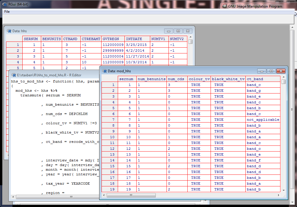
And the next slide shows another use. You see a view
of the first few lines of a raw FRS households file, a view of them after
transformation into a more convenient form, and the code that
transforms them.
Transforming Data: mutate V
Transforming Data: Filtering, Splitting, and Mutating
# mortgages_to_mod_hh_fields.R
#
# Calculates a mod_household's
# outstanding_mortgage,
# mort_interest, and mort_payment
# fields.

library( tidyverse )

library( assertthat )


mortgages_to_mod_hh_fields <- function( mortgages, params )
{
  # This function separates mortgages into two
  # sets: repayment mortgages, for which INTPRPAY > 0;
  # and interest-only mortgages, for which MORINPAY > 0.
  # In the repayment mortgages, interest is calculated from
  # payment, but in the interest-only mortgages, payment is
  # calculated from interest. The data flows in opposite
  # directions, which makes these hard to implement inside
  # a single mutate. That's why I've split them into the
  # two sets, which I process separately and then recombine
  # the results from. This may not be the most efficient
  # method, but I can optimise once we've tested it and
  # I'm sure I have the logic right.

  assert_that( ! any( mortgages$INTPRPAY > 0 & mortgages$MORINPAY > 0 ) )
  #
  # The 2014-15 data (on which I developed this code)
  # doesn't have any mortgages where both these fields
  # are greater than 0. But check anyway, for the benefit of
  # other data sets. If we find such data, we either have
  # to decree it invalid, or modify this function.

  per_repayment_mortgage_fields <- mortgages %>%
    filter( INTPRPAY > 0 ) %>%
    repayment_mortgages_to_per_mortgage_fields( params )

  per_interest_only_mortgage_fields <- mortgages %>%
    filter( MORINPAY > 0 ) %>%
    interest_only_mortgages_to_per_mortgage_fields

  per_mortgage_fields <-
    bind_rows( per_repayment_mortgage_fields
             , per_interest_only_mortgage_fields
             )

  per_hh_fields <- per_mortgage_fields %>%
    group_by( sernum ) %>%
    summarise( mort_interest=sum( mort_interest )
             , mort_payment=sum( mort_payment )
             , outstanding_mortgage = sum( outstanding_mortgage )
             ) %>%
    ungroup()

  per_hh_fields
}


repayment_mortgages_to_per_mortgage_fields <- function( mortgages, params )
{
  per_mortgage_fields <- mortgages %>%
    transmute( sernum = SERNUM

             , mort_payment = INTPRPAY

             , years_to_run = MORTEND

             , outstanding = MORTLEFT

             , interest_rate = getp( params, mortgage_rate, year, month )

             , mort_interest = calc_mortgage_interest( mort_payment,
                                                       years_to_run,
                                                       outstanding,
                                                       interest_rate )

             , outstanding_mortgage = outstanding

             )

  per_mortgage_fields
}


interest_only_mortgages_to_per_mortgage_fields <- function( mortgages )
{
  assert_that( ! any( mortgages$MORINUS == 1 & mortgages$MORUS > 0 ) )
  #
  # The case_when below assumes these two
  # conditions are distinct, so check that
  # this holds.

  per_mortgage_fields <- mortgages %>%
    transmute( sernum = SERNUM

             , mort_interest = case_when( MORINUS == 1 ~ MORINPAY
                                        , MORUS > 0    ~ MORUS
                                        , TRUE         ~ 0
                                        )

             , mort_payment = mort_interest

             , outstanding_mortgage = 0

             )

  per_mortgage_fields
}
Transforming Data: Filtering, Splitting, and Mutating II
There are places in the model where it seems convenient
to separate data into different sets of rows, process
each in its own way, and then recombine them. The code on
the previous slide is one of these. The FRS data has
two kinds of mortgage: repayment, and interest-only. Payments and
interest are calculated in very different ways.
That code is some of the most complex I’ve shown so far.
It uses grouping and summarising and recoding, which I’ve not yet
discussed. But here, the filtering and splitting is the point.
Transforming Data: Filtering, Splitting, and Mutating III
The design of R means we may filter and split where in other
languages, we’d use conditionals. The loop “for each row R, if row is type
A, process as A, else process as B” may be better written as
“Split rows into type A and type B, process each, then recombine”. There
are strangenesses about how R’s implicit looping interacts
with conditional expressions that don’t make such
a decision
straightforward. It needs careful thought about timing, about whether
arguments are single items or entire column vectors, and about
how much implicit looping R is doing.
Transforming Data: Summarising
The summarise function is great for
probing data. But sometimes, we need it for transformation too.
As already mentioned, our transformed households
contain the sum of salaries of all wage-earners in
the household. I use summarise
for that.
The function can also be used for things we wouldn’t normally
think of as aggregation. As well as summing a
household’s salaries,
we need to store a list of them in the household.
The R function list collects items into
lists: by passing that to summarise,
we can list all the items in a group.
Transforming Data: Recoding
Many FRS variables are numbers but represent
discrete attributes such as sex. So to make our transformed data more
readable, we must recode them as strings.
I’ve implemented a “coding frames” library, which
lets translation tables be defined and used as if they
were Python dictionaries. I gave an example
for the HHETHGR3 histograms
when demonstrating
plotting.
Actually, strings are not the best way to represent discrete
attributes. That’s because R won’t check for
rubbish such as mal, hemale,
or 08bnv-6b)%)$*%=856
being assigned to them. Bad stuff can get into the program and you
won’t notice.
I need to think about this: other
kinds of value, such as R “factors” (which I mentioned when doing violin
plots), may be better.
Transforming Data: Spreading and Gathering

Transforming Data: Spreading and Gathering II
To “spread”, in the Tidyverse, is to transform
a long narrow table to a short wide one. Given
a column of values and another column which
associates a type with each value, spread
makes a new column for each type, and puts each
type’s values into its column.
I use spread to classify incomes into
different categories. It is very convenient that this
can be done by just one function.
There is a gather function which
undoes spread. It takes a table with
columns for different types of value, and merges
these into one column.
Transforming Data: Nesting
Nesting, yet another Tidyverse feature, makes it possible
to put data frames into the cells of other data frames. I shan’t
demonstrate, as there isn’t a good way to display nested tables.
But they may be useful.
For example, households are composed of
benefit units: an adult plus spouse if any, plus children. And benefit
units
are composed of adults. (And children, but they’re less important.)
My code may be easier to write and read if I
store adults inside benefit units inside households, rather than
as separate tables to be JOINed. It may make
“uprating” easier, where we traverse tables updating money values to
account for
inflation.
Representation-Independent Selectors
|
|
||||||||||||||||||||||||||||||||||||||||
|
|
Representation-Independent Selectors II
“In the early stages of NIPY development, we focus on
functionality
and usability. As NIPY progresses,
we will spend more energy on optimizing critical functions.
There are many good options, including standard
C-extensions. However, optimized code is often less readable and more
difficult to debug and maintain. When we do optimize, we will
first profile the code to determine the offending sections, then optimize
those.” Abridged from
http://nipy.org/nipy/devel/guidelines/optimization.html .
“First make it work. Then make it right. Then make it fast.”
Attributed to Kent Beck.
“We should forget about small efficiencies, say about 97% of the
time: premature optimization is the root of all evil.”
Donald Knuth.
Representation-Independent Selectors III
“When you start development, you have an early stage where you
need
to explore possibilities. You
don’t yet know the best approach,
but have some ideas. If during that stage you go big looking for THE piece
of code that will fit the problem perfectly, you will spend a
considerable amount of time on that quest. You
have too
many uncertainties. So you need to
experiment to reduce those uncertainties, so
you can focus and implement your code. This experimentation process is the
Make it Work stage, where you just code to achieve the desired behavior or
effect.” Abridged from
http://henriquebastos.net/the-make-it-work-make-it-right-make-it-fast-misconception/
.
Representation-Independent Selectors IV
So when we begin coding, we must experiment to find more about possible
solutions. Near the end of coding, we may need to optimise. But experiment
and optimisation can both mean big changes to data structures. Some of
these are made possible by nesting; and as the first slide shows, there
are many ways to store the same information.
But when we change how data is stored, we don’t want to change all the
code that accesses it! Which we would if we relied on $ and column names:
consider how different the expressions would be for retrieving Bob’s
benefits in each of the four layouts on the first slide.
Representation-Independent Selectors and Model Parameters
This
applies not only to household data, but
to the “parameters” that drive the model. These describe
the taxes, and include
stuff like VAT rates on a vast range of goods.
The Python version stored different parameters differently.
Some to be accessed via subscripting with strings; some via subscripting
with integers; some via dictionary keys. Change storage, and
you’d have to update all the access code.
Representation-Independent Selectors V
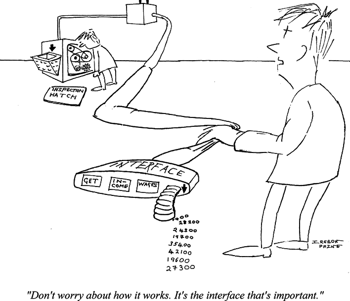
My solution rests on two things. First, do all accesses
via functions that I define, rather than via $
and column names. Then if I ever change the storage, I can update
those functions accordingly. This provides an interface to
data that’s
independent of its representation.
Second, R and the Tidyverse provide features for changing how
the language processes the arguments to functions. With these,
we can make string subscripts look like column names. This hides
the differences between different kinds of selector. So if we change
storage, it’s
easier to change what they select from.
Representation-Independent Selectors VI
Towards R-Taxben: Reading Parameters
Towards R-Taxben: Reading Parameters II
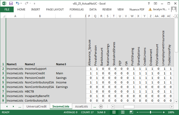
The model parameters are held in spreadsheets. To
read these, I use the read_excel
function from the Tidyverse “readxl” package. It
handles Excel files directly, without them having to be
converted to CSV.
The function returns a data frame. I have to convert
the names in the three columns on the left,
so that the rest of the model
can ask questions like “What’s the
value of parameter Savings in PensionCredit in IncomeLists?”
I wrote a function called multinest
for this, which turns the names into a list of
lists of lists. The model could then get at
parameters using
$ and column names, in expressions
like IncomeLists$PensionCredit$Savings .
Towards R-Taxben: Reading Parameters III
But as discussed, an expression like
IncomeLists$PensionCredit$Savings
is fragile. If
I change parameter representation, I’d have to recode it.
So I wrote a function getp, which insulates
its user from the representation. I call it
like this:
getp( IncomeLists, PensionCredit, Savings ) .
If I change the representation, I redefine getp,
and the user should notice no difference.
Towards Program Quality: Experiments

Towards Program Quality: Experiments II
“When you start development, you have an early stage where you need to
explore possibilities. … So you need to
experiment to reduce those uncertainties, so you can focus and implement
your code. This experimentation process is the Make it Work stage, where
you just code to achieve the desired behavior or effect.”
Quoted earlier under Representation-Independent Selectors,
abridged from
http://henriquebastos.net/the-make-it-work-make-it-right-make-it-fast-misconception/ .
I keep my experiments, commented so that I and others can
read them easily. Because they may be useful later. As we’ll see, I also
blog some of them.
Towards Program Quality: Readable Code
# Returns a family_type. See the
# family_type document.
# age_2 and sex_2 are only defined
# if is_couple .
#
family_type <- function( age_1, sex_1
                       , age_2, sex_2
                       , is_couple
                       , num_children
                       )

{
  ad1_is_pensioner <- of_pensionable_age( age_1, sex_1 )
  ad2_is_pensioner <- of_pensionable_age( age_2, sex_2 )

  is_single <- !is_couple

  case_when(
    is_couple & ( ad1_is_pensioner | ad2_is_pensioner ) ~ 'couple_pensioner'
  , is_single & ad1_is_pensioner                        ~ 'single_pensioner'
  , is_couple & num_children == 0                       ~ 'couple_no_children'
  , is_single & num_children == 0                       ~ 'single_no_children'
  , is_couple & num_children > 0                        ~ 'couple_children'
  , is_single & num_children > 0                        ~ 'single_children'
  )
}
Towards Program Quality: Readable Code II
The slide before shows a function that
indicates what kind of family a benefit unit contains, for
the purposes of their benefits. For example,
pensioners receive pensions, so it has to use age to work out
whether the adults are pensioners. Children receive
child benefit, so it has to say whether the family includes
children.
I have tried to make this as readable as possible. That’s
essential for maintenance, especially when the code
is handling complicated things. Like the UK benefits
system.
A Reference Standard for UK Benefits
The UK benefits system is notoriously opaque.
This helps the Government save money, by making it harder
to understand what you can claim. But although the
Government has no interest in clarity,
organisations that help claimants do. For example, the
Childhood Poverty Action Group publishes its
Welfare
Benefits and Tax Credits Handbook: “an essential resource for all
professional advisers serious about giving the best and most accurate
advice to their clients”.
It would be great if R-Taxben could
become accepted as a reference standard for the benefits system, against
which interpretations of the benefits rules could be tested: an electronic
Handbook. We think this is feasible. It will
require
our code to be very very readable.
Towards Program Quality: Testing
# test_utilities.R
#
# Test the functions in utilities.R


library( testthat )

source( 'utilities.R' )


test_that( "year_and_month_to_tax_year() works", {

  expect_that( year_and_month_to_tax_year( 1990, 1 ), equals("1989-90") )

  expect_that( year_and_month_to_tax_year( 1990, 3 ), equals("1989-90") )

  expect_that( year_and_month_to_tax_year( 1990, 4 ), equals("1990-91") )

  expect_that( year_and_month_to_tax_year( 1990, 12 ), equals("1990-91") )


  expect_that( year_and_month_to_tax_year( 2001, 1 ), equals("2000-01") )

  expect_that( year_and_month_to_tax_year( 2001, 3 ), equals("2000-01") )

  expect_that( year_and_month_to_tax_year( 2001, 4 ), equals("2001-02") )

  expect_that( year_and_month_to_tax_year( 2001, 12 ), equals("2001-02") )


  expect_that( year_and_month_to_tax_year( 2000, 1 ), equals("1999-00") )

  expect_that( year_and_month_to_tax_year( 2000, 3 ), equals("1999-00") )

  expect_that( year_and_month_to_tax_year( 2000, 4 ), equals("2000-01") )

  expect_that( year_and_month_to_tax_year( 2000, 12 ), equals("2000-01") )
  #
  # I don't know what Howard would like returned
  # for the tax year 1999-2000. This is my
  # interpretation.

  expect_that( year_and_month_to_tax_year( 1999, 1 ), equals("1998-99") )

  expect_that( year_and_month_to_tax_year( 1999, 3 ), equals("1998-99") )

  expect_that( year_and_month_to_tax_year( 1999, 4 ), equals("1999-00") )

  expect_that( year_and_month_to_tax_year( 1999, 12 ), equals("1999-00") )

})
Towards Program Quality: Testing II
# test_read_params_from_excel.R
#
# Tests params_read_table_from_excel().

library(tidyverse)
library(testthat)

source( 'read_params_from_excel.R' )


test_that( "Reads a parameter sheet and returns the expected
contents, checked in detail", {

  t <- params_read_table_from_excel(
'tests/data/v01_25_ActualNoUC.xlsx', 'CouncilTax' )

  expect_that( nrow(t), equals(24) )

  expect_that( ncol(t), equals(32) )

  expect_that( names(t)[[4]], equals('Uprating') )

  years <- 2003:2030
  year_names <- str_c( years, "-", str_sub( years+1, 3, 4 ) )
  # What the names should be: 2003-04 to 2030-31.

  expect_that( names(t)[5:ncol(t)], equals(year_names) )

  expect_that( unique(t[[1]]), equals("CouncilTax") )

  expect_that( unique(t[1:3,2][[1]]), equals("Multiplier") )

  expect_that( unique(t[4:12,2][[1]]), equals("BandMultiplier")
)

  expect_that( unique(t[13:24,2][[1]]), equals("BandDAverage") )

  expect_that( unique(str_sub(unlist(t[4:12,3]),1,4)),
equals("Band") )

  expect_that( t[[24,3]], equals("NI") )

  expect_that( unique(t[4:12,4][[1]]), equals("Repeat") )

  expect_that( unique(t[13:23,4][[1]]), equals("0.04") )
  # Although Excel displays it as 4.0%.

  expect_that( t[[24,4]], equals("PrevSep.CPI.AnnualGrowth") )

  expect_that( unique(t[3,5:31][[1]]), equals(0.75,tolerance=0.000001) )

  expect_that( unique(t[11,5:31][[1]]), equals(2.0,tolerance=0.000001) )

  expect_that( t[[24,32]], equals(1192.03,tolerance=0.000001) )

})


test_that( "Reads all the parameter sheets and passes them as
valid", {

  param_sheetnames <-
    c("General", "IncomeTax", "NICs",
"VAT", "Excise", "OtherIndirect"
     ,"CouncilTax", "IncomeSupport",
"HBCTB", "PensionCredit", "CitizensIncome"
     ,"IncapacityBenefit", "ESA",
"OtherDisabilityBenefits", "ChildBenefit"
     ,"OtherNonMTBenefits", "Winter Fuel",
"TaxCredits", "UniversalCredit"
     )
  param_sheetnames <- setdiff( param_sheetnames, "VAT" )
  #
  # The VAT sheet has a bad column heading for
  # 1999-2000, presumably caused by someone
  # misprogramming the millennium change, so I've
  # removed its name from the above. All the rest
  # should be parameter sheets in the expected
  # format.

  for ( sheetname in param_sheetnames ) {

    t <- params_read_table_from_excel(
'tests/data/v01_25_ActualNoUC.xlsx', sheetname )

    warnings <- attributes( t )$validation

    expect_that( warnings, equals( c() ) )
  }

})


# Used below to shorten the tests that check
# validation of faulty worksheets.
#
test_validation_failure <- function( title, filename, message )
{
  test_that( title, {

    t <- params_read_table_from_excel( filename, 'CouncilTax' )

    warnings <- attributes( t )$validation

    expect_that( length(warnings), equals(1) )

    expect_that( warnings[[1]], equals(message) )

})
}


test_validation_failure( "Detects bad year-column names in parameter
sheet (I)"
                       ,
'tests/data/v01_25_ActualNoUC_bad_year_colname_I.xlsx'
                       , 'Columns 8 onwards are all expected to be headed
by year numbers such as 2003-04.'
                       )
                       # First year column name is 2003-EE.


test_validation_failure( "Detects bad year-column names in parameter
sheet (II)"
                       ,
'tests/data/v01_25_ActualNoUC_bad_year_colname_II.xlsx'
                       , 'Columns 8 onwards are all expected to be headed
by year numbers such as 2003-04.'
                       )
                       # Final year column name is EE.


test_validation_failure( "Detects bad 'Name' column name in parameter
sheet"
                       ,
'tests/data/v01_25_ActualNoUC_bad_name_colname.xlsx'
                       , "Columns 4, 5, 6 and 7 are expected to be
headed 'Name', 'Uprating', 'Worksheet', and 'Lookup'."
                       )
                       # Column name is EE.


test_validation_failure( "Detects bad 'Uprating' column name in
parameter sheet"
                       ,
'tests/data/v01_25_ActualNoUC_bad_uprating_colname.xlsx'
                       , "Columns 4, 5, 6 and 7 are expected to be
headed 'Name', 'Uprating', 'Worksheet', and 'Lookup'."
                       )
                       # Column name is EE.


test_validation_failure( "Detects bad 'Worksheet' column name in
parameter sheet"
                       ,
'tests/data/v01_25_ActualNoUC_bad_worksheet_colname.xlsx'
                       , "Columns 4, 5, 6 and 7 are expected to be
headed 'Name', 'Uprating', 'Worksheet', and 'Lookup'."
                       )
                       # Column name is EE.


test_validation_failure( "Detects bad 'Lookup' column name in
parameter sheet"
                       ,
'tests/data/v01_25_ActualNoUC_bad_lookup_colname.xlsx'
                       , "Columns 4, 5, 6 and 7 are expected to be
headed 'Name', 'Uprating', 'Worksheet', and 'Lookup'."
                       )
                       # Column name is EE.


test_validation_failure( "Detects non-empty rows under column names
in parameter sheet (I)"
                       ,
'tests/data/v01_25_ActualNoUC_rows_under_colnames_not_blank_I.xlsx'
                       , "The second two rows of columns 1:3 are
expected to be empty."
                       )
                       # Top-left cell is EE.


test_validation_failure( "Detects non-empty rows under column names
in parameter sheet (II)"
                       ,
'tests/data/v01_25_ActualNoUC_rows_under_colnames_not_blank_I.xlsx'
                       , "The second two rows of columns 1:3 are
expected to be empty."
                       )
                       # Bottom-right cell is EE.


test_validation_failure( "Detects bad cell in first names column in
parameter sheet (I)"
                       ,
'tests/data/v01_25_ActualNoUC_bad_col1_name_cell_I.xlsx'
                       , "Rows 4 onwards of column 1 are expected to
be parameter names."
                       )
                       # First cell is blank.


test_validation_failure( "Detects bad cell in first names column in
parameter sheet (II)"
                       ,
'tests/data/v01_25_ActualNoUC_bad_col1_name_cell_II.xlsx'
                       , "Rows 4 onwards of column 1 are expected to
be parameter names."
                       )
                       # Final cell is blank.


test_validation_failure( "Detects bad cell in first names column in
parameter sheet (III)"
                       ,
'tests/data/v01_25_ActualNoUC_bad_col1_name_cell_III.xlsx'
                       , "Rows 4 onwards of column 1 are expected to
be parameter names."
                       )
                       # Final cell is a number.


test_validation_failure( "Detects bad cell in second names column in
parameter sheet (I)"
                       ,
'tests/data/v01_25_ActualNoUC_bad_col2_name_cell_I.xlsx'
                       , "Rows 4 onwards of column 2 are expected to
be parameter names or empty."
                       )
                       # First cell is a number.


test_validation_failure( "Detects bad cell in second names column in
parameter sheet (II)"
                       ,
'tests/data/v01_25_ActualNoUC_bad_col2_name_cell_II.xlsx'
                       , "Rows 4 onwards of column 2 are expected to
be parameter names or empty."
                       )
                       # Final cell ends in '#'.


test_validation_failure( "Detects bad cell in third names column in
parameter sheet (I)"
                       ,
'tests/data/v01_25_ActualNoUC_bad_col3_name_cell_I.xlsx'
                       , "Rows 4 onwards of column 3 are expected to
be parameter names or empty."
                       )
                       # First cell is 'Gener@l'.


test_validation_failure( "Detects bad cell in third names column in
parameter sheet (II)"
                       ,
'tests/data/v01_25_ActualNoUC_bad_col3_name_cell_II.xlsx'
                       , "Rows 4 onwards of column 3 are expected to
be parameter names or empty."
                       )
                       # Final cell is 'N I'.


test_that( "The params_string_matches_year() function works", {

  expect_that( params_string_matches_year(''), is_false() )

  expect_that( params_string_matches_year('EE'), is_false() )

  expect_that( params_string_matches_year('2003'), is_false() )

  expect_that( params_string_matches_year('2003-'), is_false() )

  expect_that( params_string_matches_year('2003-EE'), is_false() )

  expect_that( params_string_matches_year('2003-0E'), is_false() )

  expect_that( params_string_matches_year('2003-04'), is_true() )

})


test_that( "The params_string_matches_year() function is
vectorised", {

  v <- c( '', 'EE', '2003', '2003-04', '2011-12', '2012-1E' )

  expected <- c( FALSE, FALSE, FALSE, TRUE, TRUE, FALSE )

  expect_that( params_string_matches_year(v), equals(expected) )

})
Towards Program Quality: Testing III
# test_benefits_to_incomes.R
#
# Test benefits_to_incomes().


library( tidyverse )

library( testthat )

source( 'functions_to_help_with_testing.R' )

source( 'benefits_to_incomes.R' )

source( 'read_frs_data_from_csv.R' )

source( 'benefit_types.R' )


test_that( "benefits_to_incomes() works", {

  benefits <- read_frs_benefits_from_csv(
"data/FRS201415AllData/benefits.csv" )

  incomes <- benefits_to_incomes( benefits )

  tol <- 1e-3


  # Test final serial number. We don't
  # necessarily use all the records, so this
  # may be less than the final serial number
  # in the original data.

  expect_lte( tail(incomes,1)$sernum, 19535 )


  # Test that after's serial numbers are a
  # subset of before's.

  expect_true( all( unique(incomes$sernum) %in% unique(benefits$SERNUM) )
)


  # Test that there is only one record
  # for each sernum/persnum combination.
  # benefits_to_incomes() aggregates
  # over all benefit records for the
  # same person, so should ensure that.

  expect_equal( incomes %>% group_by( sernum, persnum ) %>%
                tally() %>%
                `$`( n ) %>%
                unique()
              , 1
              )


  # Test column names.

  expect_equal( names(incomes)
              , c( 'sernum', 'persnum', benefit_types() )
              )


  # Test contents of benefit-type cells.

  expect_equal( at_sernum( incomes, 1, child_benefit )
              , 47.6, tolerance=tol
              )

  expect_equal( at_sernum( incomes, 1, child_tax_credit )
              , 40.055, tolerance=tol
              )

  expect_equal( at_sernum( incomes, 1, pip_care )
              , 0
              )
  # 0 because there was no record for it,
  # but there were others for other
  # benefit types for this person.

  expect_equal( at_sernum( incomes, 3, retirement_pension )
              , 125.9041096, tolerance=tol
              )

  expect_equal( at_sernum( incomes, 3, winter_fuel_payment )
              , 150, tolerance=tol
              )

  expect_equal( at_sernum( incomes, 3, last_6m_child_maintenance )
              , 0
              )
  # 0 because there was no record for it,
  # but there were others for other
  # benefit types for this person.

  expect_equal( at_sernum( incomes, 3, retirement_pension )
              , 125.9041096, tolerance=tol
              )

  expect_equal( at_sernum( incomes, 3, winter_fuel_payment )
              , 150, tolerance=tol
              )

  expect_equal( at_sernum( incomes, 3, retirement_pension, 2 )
              , 67.8136986, tolerance=tol
              )

  expect_equal( at_sernum( incomes, 3, winter_fuel_payment, 2 )
              , 150, tolerance=tol
              )

  expect_equal( at_sernum( incomes, 3, guardians_allowance, 2 )
              , 0
              )
  # 0 because there was no record for it,
  # but there were others for other
  # benefit types for this person.


})
Towards Program Quality: Testing IV
test_that( "family_type() works", {

  expect_that( family_type( 59, 'male', NA, NA, FALSE, 0 )
             , equals('single_no_children')
             )

  expect_that( family_type( 59, 'female', NA, NA, FALSE, 0 )
             , equals('single_no_children')
             )

  expect_that( family_type( 59, 'male', NA, NA, FALSE, 1 )
             , equals('single_children')
             )

  expect_that( family_type( 59, 'female', NA, NA, FALSE, 1 )
             , equals('single_children')
             )


  expect_that( family_type( 60, 'male', NA, NA, FALSE, 0 )
             , equals('single_no_children')
             )

  expect_that( family_type( 60, 'female', NA, NA, FALSE, 0 )
             , equals('single_pensioner')
             )

  expect_that( family_type( 60, 'male', NA, NA, FALSE, 1 )
             , equals('single_children')
             )

  expect_that( family_type( 60, 'female', NA, NA, FALSE, 1 )
             , equals('single_pensioner')
             )


  expect_that( family_type( 64, 'male', NA, NA, FALSE, 0 )
             , equals('single_no_children')
             )

  expect_that( family_type( 64, 'female', NA, NA, FALSE, 0 )
             , equals('single_pensioner')
             )

  expect_that( family_type( 64, 'male', NA, NA, FALSE, 1 )
             , equals('single_children')
             )

  expect_that( family_type( 64, 'female', NA, NA, FALSE, 1 )
             , equals('single_pensioner')
             )


  expect_that( family_type( 65, 'male', NA, NA, FALSE, 0 )
             , equals('single_pensioner')
             )

  expect_that( family_type( 65, 'female', NA, NA, FALSE, 0 )
             , equals('single_pensioner')
             )

  expect_that( family_type( 65, 'male', NA, NA, FALSE, 1 )
             , equals('single_pensioner')
             )

  expect_that( family_type( 65, 'female', NA, NA, FALSE, 1 )
             , equals('single_pensioner')
             )


  expect_that( family_type( 59, 'male', 59, 'female', TRUE, 0 )
             , equals('couple_no_children')
             )

  expect_that( family_type( 59, 'female', 59, 'male', TRUE, 0 )
             , equals('couple_no_children')
             )

  expect_that( family_type( 59, 'male', 59, 'female', TRUE, 1 )
             , equals('couple_children')
             )

  expect_that( family_type( 59, 'female', 59, 'male', TRUE, 1 )
             , equals('couple_children')
             )


  expect_that( family_type( 60, 'male', 60, 'female', TRUE, 0 )
             , equals('couple_pensioner')
             )

  expect_that( family_type( 60, 'female', 60, 'male', TRUE, 0 )
             , equals('couple_pensioner')
             )

  expect_that( family_type( 60, 'male', 60, 'female', TRUE, 1 )
             , equals('couple_pensioner')
             )

  expect_that( family_type( 60, 'female', 60, 'male', TRUE, 1 )
             , equals('couple_pensioner')
             )


  expect_that( family_type( 60, 'male', 59, 'female', TRUE, 0 )
             , equals('couple_no_children')
             )

  expect_that( family_type( 59, 'female', 60, 'male', TRUE, 0 )
             , equals('couple_no_children')
             )

  expect_that( family_type( 60, 'male', 59, 'female', TRUE, 1 )
             , equals('couple_children')
             )

  expect_that( family_type( 59, 'female', 60, 'male', TRUE, 1 )
             , equals('couple_children')
             )


  expect_that( family_type( 65, 'male', 59, 'female', TRUE, 0 )
             , equals('couple_pensioner')
             )

  expect_that( family_type( 59, 'female', 65, 'male', TRUE, 0 )
             , equals('couple_pensioner')
             )

  expect_that( family_type( 65, 'male', 59, 'female', TRUE, 1 )
             , equals('couple_pensioner')
             )

  expect_that( family_type( 59, 'female', 65, 'male', TRUE, 1 )
             , equals('couple_pensioner')
             )


  expect_that( family_type( 65, 'male', 65, 'female', TRUE, 0 )
             , equals('couple_pensioner')
             )

  expect_that( family_type( 65, 'female', 65, 'male', TRUE, 0 )
             , equals('couple_pensioner')
             )

  expect_that( family_type( 65, 'male', 65, 'female', TRUE, 1 )
             , equals('couple_pensioner')
             )

  expect_that( family_type( 65, 'female', 65, 'male', TRUE, 1 )
             , equals('couple_pensioner')
             )

})


test_that( "of_pensionable_age() works", {

  expect_that( of_pensionable_age( 1, 'male' ), is_false() )
  expect_that( of_pensionable_age( 1, 'female' ), is_false() )

  expect_that( of_pensionable_age( 20, 'male' ), is_false() )
  expect_that( of_pensionable_age( 20, 'female' ), is_false() )

  expect_that( of_pensionable_age( 59, 'male' ), is_false() )
  expect_that( of_pensionable_age( 59, 'female' ), is_false() )

  expect_that( of_pensionable_age( 60, 'male' ), is_false() )
  expect_that( of_pensionable_age( 60, 'female' ), is_true() )

  expect_that( of_pensionable_age( 64, 'male' ), is_false() )
  expect_that( of_pensionable_age( 64, 'female' ), is_true() )

  expect_that( of_pensionable_age( 65, 'male' ), is_true() )
  expect_that( of_pensionable_age( 65, 'female' ), is_true() )

  expect_that( of_pensionable_age( 100, 'male' ), is_true() )
  expect_that( of_pensionable_age( 100, 'female' ), is_true() )

})
Towards Program Quality: Testing V
I use the package “testthat” for testing.
To use it, you write a collection of function calls
or other expressions, each with a statement of
what its result should be. The package runs each one
and reports an error if its result is not as
expected.
Towards Program Quality: Testing VI
The first slide tests the simple function
year_and_month_to_tax_year shown
earlier.
Towards Program Quality: Testing VII
The second slide tests reading
parameter spreadsheets. It starts by checking
the size of the read data and the contents
of cells. It then sees whether it can read all
our parameter sheets. Then it checks a collection
of erroneous spreadsheets I made, testing that the
error messages from each are as expected. Finally, it
tests one of the functions used, one for matching against
tax years in column headings.
Rigorous testing — for example,
preparing all those faulty spreadsheets — is a lot
of work!
Towards Program Quality: Testing VIII
The third slide tests conversion of
FRS benefits data to incomes. There are some
general tests on IDs and data structure, followed by
detailed tests on fields in converted records.
In these tests, I had to think about missing
data and how it’s aggregated. For example, what should
the results be if a
person has no benefits records at all? What if they
have records for some benefits but not for others?
Towards Program Quality: Testing IX
The fourth slide tests the family_type
function and another function it calls, of_pensionable_age.
It needs to test a lot of combinations, of ages above, below, and on
the pension thresholds.
Towards Program Quality: Profiling

Towards Program Quality: Profiling II
Profilers show time spent
or memory used in different regions of a program. They help you
focus on the parts that need optimising. The screenshot
is a profile output by the “profvis” package. It’s for a function I
wrote that generates sample children to inhabit households,
in order to test using household and people tables together.
Towards Program Quality: Benchmarking

Towards Program Quality: Benchmarking II
Benchmarking tests the performance of code,
often by comparing with alternative versions.
The screenshot is output from the “microbenchmark”
package. It’s comparing the times to run
four versions of my function spread_to_list,
called when reading the hierarchical names from
parameter worksheets. Two versions of the function
were much slower than the other two, so I didn’t
need to develop them further. The other two were
about the same speed, so it didn’t matter
which one I used.
Towards Program Quality: Documentation
I am documenting all the
data structures my code uses, with a
a web page describing each structure.
This alleviates the problem that in R, any variable can
hold any type of data. Unlike e.g. Pascal, which requires
every variable to be declared with one and only one type.
That type helps the compiler check that wrong kinds of
data aren’t getting into the variable. It is also useful documentation
for the reader. But in R, the compiler can’t check,
and it’s easy to make mistakes. So I need to comment
every variable with details of what it holds.
But to avoid writing everything about a type in every comment
that refers to it, we need to centralise the information.
That’s what my documentation pages do.
Towards Program Quality: Documentation II
R has features not found in other languages. Implicit
looping over vectors is one. Another is “NA” values, used
for when data is missing. We have to consider these when
documenting. For a function, we need to say whether it
does implicit looping or not. Some don’t. For data, we
have to say whether it contains NA values, and when, and
exactly what they signify. You can see that the latter
needs a lot of care.
Towards Program Quality: Blogging
We hope R-Taxben will become open-source,
so that people everywhere can collaborate on it.
But even if that doesn’t happen, it’s important to have
a record not only of how the code works, but of why
it was designed to work that way. I am providing this
by blogging about my design.
I could have written just for myself. But blogging
keeps me honest, making me explain clearly to other people.
It brings R-Taxben to the attention of people who
might use it or collaborate. And some posts may
help R programmers with other programs.
The next slide lists my posts to date, 14th March 2018.
To see all posts, go to http://www.j-paine.org/blog/
and select those categorised under “R”.
Towards Program Quality: Blogging II
Two
Kinds of Conditional Expression: ifelse(A,B,C) versus if (A) B else
C
One out of quite a lot of confusing things about R is that it has two
kinds of conditional expression. There’s ifelse(); and there’s
the if statement. It’s important to know which one to use, as I
found when trying to write a conditional expression that chose between
lists. The first thing to appreciate is … Continue reading
“Two Kinds of Conditional Expression: ifelse(A,B,C) versus if (A) B
else C”
Beat
the Delays: installing R and the BH package on a memory stick
I use R on a range of Windows machines. Often, I’ll only use these
once, and they won’t already have R. So I want to carry an
installation with me. So I decided to install R on a memory stick.
Installing R itself worked, once I’d changed the folder on the
“Select Destination Location” pop-up. … Continue reading
“Beat the Delays: installing R and the BH package on a memory
stick”
Experiments
with count(), tally(), and summarise(): how to count and sum and list
elements of a column in the same call
Most people have a job. Some don’t. And a few have more than one.
I’ve mentioned before that our economic model works on data about
British households, gathered from surveys such as the Family Resources
Survey. Each collection of data is a year long, and contains a file that
describes all the adults in the … Continue reading
“Experiments with count(), tally(), and summarise(): how to count
and sum and list elements of a column in the same
call”
Second-Guessing
R
I keep doing experiments with R, and with its Tidyverse package, to
discover whether these do what I think they’re doing. Am I justified
in spending the time? I’ve said before that the Tidyverse follows
rather different conventions from those of base R. This is something Bob
Muenchen wrote about in “The Tidyverse Curse”. Dare …
Continue reading
“Second-Guessing R”
Experiments
with summarise(); or, when does x=x[[1]]?
Here’s another innocent-eye exploration, this time about the
Tidyverse’s summarise() function. I’d been combining data
tables by nesting and joining them, which gave me a tibble with nested
tibbles in. I wanted to check the sizes of these inner tibbles, by mapping
nrow() over the columns containing them. The Tidyverse provides several
ways to do … Continue reading
“Experiments with summarise(); or, when does
x=x[[1]]?”
My
Testing Was Hurt By a List With No Names
I spied a strange thing with my innocent eye. I was testing
spread_to_list, the function I wrote about in “How Best to Convert a
Names-Values Tibble to a Named List?”. One of my tests passed it a
zero-row tibble, expecting that the result would be a zero-element list:
test_that( “Test on zero-element tibble”, { t … Continue reading
“My Testing Was Hurt By a List With No Names”
Multinest:
Factoring Out Hierarchical Names by Converting Tibbles to Nested Named
Lists
Consider this tibble: vat_rates <- tribble( ~l1, ~l2 , ~l3 , ~val ,
‘VAT’, ‘Cigarettes’, ” ,
‘standard’ , ‘VAT’, ‘Tobacco’ ,
” , ‘standard’ , ‘VAT’,
‘Narcotics’ , ” , 0 , ‘VAT’,
‘Clothing’ , ‘Adult’ , ‘standard’ ,
‘VAT’, ‘Clothing’ , ‘Children’ , 0 ,
‘VAT’, ‘Clothing’ , ‘Protective’, 0 )
It contains … Continue reading
“Multinest: Factoring Out Hierarchical Names by Converting Tibbles
to Nested Named Lists”
How
Best to Convert a Names-Values Tibble to a Named List?
Here, in the spirit of my “Experiments with by_row()” post,
are some experiments in writing and timing a function spread_to_list that
converts a two-column tibble such as: x 1 y 2 z 3 t 4 to a named list:
list( x=1, y=2, z=3, t=4 ) I need this for processing the parameter sheets
shown in … Continue reading
“How Best to Convert a Names-Values Tibble to a Named
List?”
Experiments
with by_row()
I’ve been experimenting with by_row() from the R purrrlyr package.
It’s a function that maps over the rows of a data frame, which I
thought might be handy for processing our economic model’s parameter
files. I didn’t find the documentation for by_row() told me
everything I wanted to know, so I made up and ran … Continue reading
“Experiments with by_row()”
Abstract
Data Types and the Uniform Referent Principle II: why Douglas T. Ross
would hate nest(), unnest(), gather() and spread()
In “Abstract Data Types and the Uniform Referent Principle I: why
Douglas T. Ross would hate nest(), unnest(), gather() and spread()”,
I explained why the notation for interfacing to a data structure should be
independent of that structure’s representation. R programmers honour
this principle in the same way that bricks hang in the sky. All …
Continue reading
“Abstract Data Types and the Uniform Referent Principle II: why
Douglas T. Ross would hate nest(), unnest(), gather() and
spread()”
Abstract
Data Types and the Uniform Referent Principle I: why Douglas T. Ross would
hate nest(), unnest(), gather() and spread()
“What’s the Uniform Referent Principle?” my colleague
asked me on reading my last post. I think I first came across it in Jean
Sammet’s famous book Programming Languages: History and
Fundamentals. In a description of Douglas Ross’s AED-0 language, she
pointed out a feature that she thought particularly noteworthy: the
notation for getting information out … Continue reading
“Abstract Data Types and the Uniform Referent Principle I: why
Douglas T. Ross would hate nest(), unnest(), gather() and
spread()”
Thoughts
on nest()
I’ve been experimenting with the Tidyverse’s nest function,
because it may be useful when, for example, using households together with
benefit units. Below are some thoughts that I first posted as a comment to
Hadley Wickham’s blog entry “tidyr 0.4.0”. More on this
in future posts. First, this is likely to be very useful to … Continue reading
“Thoughts on nest()”
Literate
Programming, Data-flow Networks, and the Inscrutability of Economic
Models
Write programs as if they were mathematical essays, but with code instead
of equations. This is “literate programming”, an idea invented
by the famous computer scientist Donald Knuth. The quote below is from
www.literateprogramming.com , apparently first published by Knuth in
“Literate Programming (1984)” in Literate Programming, CSLI,
1992, page 99: I believe that the … Continue reading
“Literate Programming, Data-flow Networks, and the Inscrutability of
Economic Models”
Viewlets
In my last post, I said that I’d arranged for the nodes in my
network diagram to be clickable. Clicking on a data node brings up a
display showing its contents plus an explanation thereof; clicking on a
transformation node shows the code it runs and an explanation of that. I
call these little displays … Continue reading
“Viewlets”
A
Web Interface for Accessing Intermediate Results in R, Using Network
Graphs with vis.js
My title says it all. I wanted to give those running our model, myself
included, a way to visualise how it works, and to access and check
intermediate results. At the top level, the model consists of a few rather
large functions sending chunks of data from one to another. These chunks
are not conceptually … Continue reading
“A Web Interface for Accessing Intermediate Results in R, Using
Network Graphs with vis.js”
Implementing
Key-Value Notation for Data Frames without Using Tribbles
There’s a lot to be said for tribbles. As Hadley Wickham says in the
“Tibbles” chapter of R for Data Science, his tribble function
makes it easy to enter small data tables in a program, because you can
type them row by row rather than column by column. Like this: tribble(
~actor , ~character, “Shatner”, … Continue reading
“Implementing Key-Value Notation for Data Frames without Using
Tribbles”
Random
Benefit Units for Households II: Generating the Number of Subrows
In my previous post, I assumed my household data would give me the number
of children each household has. But suppose I had to generate those
numbers too? This is just a note to say that one can do this using the
base-R function sample.int . If I understand its documentation correctly,
then the call … Continue reading
“Random Benefit Units for Households II: Generating the Number of
Subrows”
Random
Benefit Units for Households I: Generating Random Subrows of a
Row
The data for our economic model comes from records representing the income
and expenditure of British households. However, the structure isn’t
as simple as just one row per household. This is because it’s
necessary to split households into “benefit units”: the word
“benefit” here refering to the money the State gives you when
you’re ill, … Continue reading
“Random Benefit Units for Households I: Generating Random Subrows of
a Row”
From
Python Dictionaries to Tribbles II: How I Implemented Lookup Tables in R
for Numeric Data Codes
In my last post, I explained how tribbles make it easy to write data
frames as a sequence of key-value pairs. But how can I make these data
frames act as lookup tables? By using the base R function match. This is
how it works. First, I’ll make a tibble: dict <- tribble( ~key,
~value, … Continue reading
“From Python Dictionaries to Tribbles II: How I Implemented Lookup
Tables in R for Numeric Data Codes”
From
Python Dictionaries to Tribbles I: How I Implemented Lookup Tables in R
for Numeric Data Codes
As regular readers will know, I’ve been translating an economic
model from Python into R. It reads data about the income and expenditure
of British households, from sources such as the Family Resources Survey
and Family Expenditure Survey . Much of this data is coded as numbers, and
the model has to translate these into … Continue reading
“From Python Dictionaries to Tribbles I: How I Implemented Lookup
Tables in R for Numeric Data Codes”
Reification
We programmers live our working lives surrounded by data structures and
subroutines, entities that become as concrete to us — as
“thing-like”, as “manipulable” — as teacups
and bricks. The feeling of thingness is strengthened, I think, by
interactive shells such as R’s which enable one to call functions
and inspect their results, and to … Continue reading
“Reification”
The
Innocent Eye, the Martian Poet, and the R Inferno
Literature has the concept of the “innocent eye”: that visitor
to regions strange who, vision unclouded by familiarity, is able to see
and report on how absurd things really are over there. There are also
“Martian poets”, who send home postcards about the oddities of
their own environment as if visiting it from Mars. As … Continue reading
“The Innocent Eye, the Martian Poet, and the R
Inferno”
Which
Symbol Should I Use for Assignment?
Perhaps I should add to my post about FreeFormatter. I noted that manual
conversion of R code for inclusion in web pages is a pain because of the
assignment symbol, <-. But I feel I should say that assignment can also
be written as =, though this sometimes clashes with = for named function
arguments. … Continue reading
“Which Symbol Should I Use for Assignment?”
FreeFormatter:
Escaping R Code for HTML
My demo of spreading and gathering data, like all my blog posts, is
written in HTML. To prevent < and > symbols in my code messing this
up, I had to “escape” them by rewriting them as < and
>. This is more of a pain in R than in many other languages,
because of … Continue reading
“FreeFormatter: Escaping R Code for HTML”
Demonstrating
spread() and gather()
In my last post about R, I said I was translating an economic model from
Python into R. It’s a microeconomic model, meaning that it simulates
the behaviour of individual people rather than bulk quantities such as
inflation and unemployment. The simulator uses data about the income and
expenditure of British households, from sources such … Continue reading
“Demonstrating spread() and gather()”
Should
I Use the Tidyverse?
I’m doing a lot of programming in the statistics language R, as I
translate an economic model into R from Python. This is a big project, and
I’ll blog about it more in later posts, as I share useful bits of
code I’ve written. But in this post, I want to mention a kind of
… Continue reading
“Should I Use the Tidyverse?”
A Web Interface
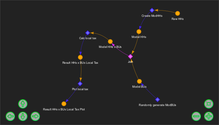
A Web Interface II: Viewing Data

A Web Interface III: Viewing Code
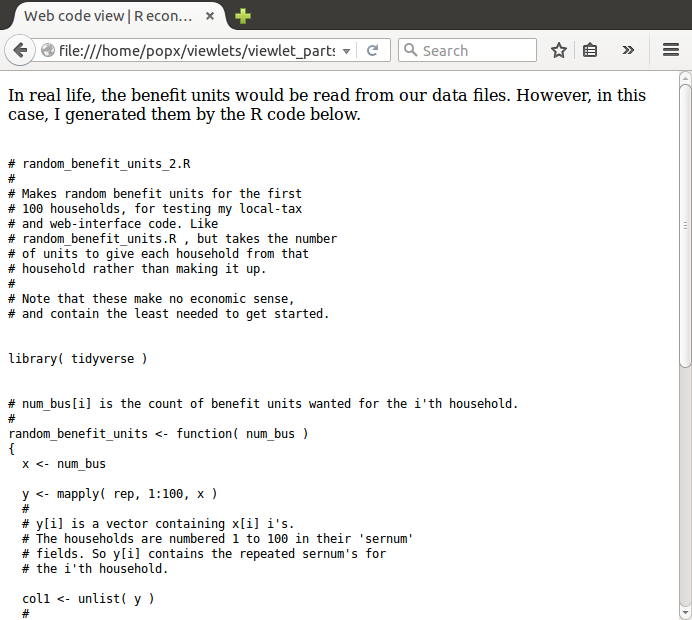
A Web Interface IV: Non-inscrutability
R can be run from a web server. The previous three slides show my web
interface, built
in Almende’s Vis.js visualisation
library.
The first slide is a network showing top-level
functions (in an older version of the model) as diamonds, and results as
circles. Lines
show how data flows between functions.
By
clicking on a
circle, the user can view the data; by clicking on an arrow, the
function code. Because data is just tables, it’s easy to understand.
It is essential that users can see how R-Taxben works.
Traditionally, economic models have been opaque, their
assumptions known only to the few who implemented them. As
we’ve seen, R programmers can probe the data using R. But
with this display, even the non-programmers are free to peer inside.
The End